Over the next few columns, we will
continue our discussion on data storage systems and look at how they are
evolving to cater to the world of data-centric computing.
Last month, we had started our discussion
of storage systems by looking at various concepts like SAN, NAS, etc. In this
column, we will look at the concept of scale-up vs. scale-out storage, and
discuss their relative advantages and disadvantages.
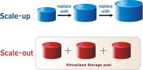
Scale-up vs. scale-out storage
Most of us are familiar with the concepts
of scale up and scale-out computing as they apply to server computing. A
scale-up server is a single system with high CPU power and huge memory, and
hence is able to handle increasing workloads. As the load on the system
increases, it can be scaled up by adding more CPUs, more memory and storage to
the single system, which is typically a shared memory system. The work is
usually done by multiple threads and processes running on the same system, and
they typically communicate through shared memory. This is a ‘shared-everything’
system. On the other hand, scale-out computing is when multiple nodes are part
of the system, and they all act together to handle the workload, which is
typically partitioned across the nodes. There is usually no shared memory
across the nodes – they communicate through explicit messages over the network.
Each node has both processing and storage elements. This is normally a ‘shared nothing’
approach, where the nodes interact in a loosely coupled manner. The scale-out
system can be scaled up to handle additional loads by adding more nodes to it;
the work can be distributed across newly added nodes transparently, without the
need to bring down the system.
The
concept of scale-up vs. scale-out storage, and discuss their relative
advantages and disadvantages
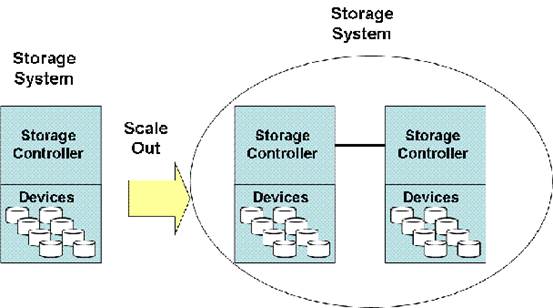
Now, scale-out and scale-up storage systems
have the same conceptual difference. In a scale-up storage system, you add more
and more storage capacity to the single storage node to meet increasing storage
requirements. This can be achieved by adding many individual disk drives to a
storage controller (or a pair of storage controllers so as to ensure failover
and high availability). Since the storage capacity (i.e., number of individual
disk drives) that a storage controller can support is limited, if storage
requirements exceed that capacity, the only option is to move to the next
bigger controller, with a higher capacity. With scale-out storage, this problem
is avoided, since each node has its own storage controller, and as you add more
nodes to meet increasing storage demands, it allows the controller architecture
to grow as well. Scale-out storage is typically marketed under the slogan, “Pay
as you grow”, since it allows you to add nodes as and when your storage requirements
increase, instead of having to over-provision from the beginning itself.
How
do scale-up and scale-out storage systems compare in terms of performance?
The next question that arises is about
performance and cost. How do scale-up and scale-out storage systems compare in
terms of performance? Before that, we need to understand what the common
measures of performance for storage systems are. For computing systems, you can
specify its performance in terms of its clock frequency (1/clock frequency gives
the clock cycle period) and Cycles Per Instruction (CPI). It is possible to
approximate the execution time for a program as (clock period * CPI *
Instruction Count). For a computation system, the number of
operations/instructions completed per second is a performance measure. This is
typically specified as how many MIPS (million instructions per second) or how
many FLOPS (floating point operations per second) the system can execute. For
storage systems, the typical performance measures used are:
1. Throughput,
2. IOPS (number of Input /Output Operations Per Second), and
3. Average latency of an operation.
The most common measure of a storage system
– be it a simple SATA drive connected directly to your PC, or a complex storage
array controller connected through SCSI – is how much maximum throughput it can
deliver. This is measured as data transfer per second (megabytes per second or
MBps). IOPS is the number of IO operations that can happen per second on the
storage device, and is defined as the total number of read/write operations
that can be performed in one second on the storage device in question. An IO
operation request will take a certain time to complete. This can be specified
in terms of average latency of an IO operation. Each IO operation is an IO request
for a certain size of IO. In simple terms, an IO request can be a read
operation of X bytes or a write operation of Y bytes. Hence, each IO request is
characterized by its type and size. Now, we can approximate the throughput/data
transferred into and out of storage systems as:
Throughput =
IOPS * average latency of IO operation * average request size
The IO request latency is limited by a
number of factors, including the physical factors associated with the storage
system. Let us consider a trivial example where the storage system is the
traditional hard disk. Here the IO latency is limited by the rotational delay
of the disk, the seek time of the disk and data transfer latency. The
rotational delay is governed by the disk’s rotational speed, which is expressed
in Revolutions Per Minute (RPM) and indicates the amount of time it takes to
get the right sector under the disk head. The seek time is governed by the time
it takes for the disk head to position itself on the right track on the disk.
Once the disk head is in the right position, it can start reading/writing the
data. The delay incurred in reading/writing the data is the data transfer
latency. All these three components contribute to the IO request latency.
Depending on the purpose of the storage
system, any or all of these performance measures would be significant. For
instance, if you are using the storage system for backup/archival purposes, you
may be more concerned with overall IO throughput rather than the individual IO
request latency. On the other hand, if the purpose is to serve data to a
latency-sensitive/client facing application such as a database, IO request
latency would become a significant measure of performance for the storage
system under consideration. Hence, different performance measures are
applicable for different workloads being deployed on the storage system.

Given
that the file access operation can span multiple nodes as in the example
mentioned earlier, let us assume that we are trying to delete the file located
at ‘/dir1/file1’ in this example
Coming back to comparing scale-out storage
and scale-up storage, each has its own performance benefits. Scale-up storage
can offer good IO request latencies, while scale-out can offer good IO
throughputs. Since scale-out storage is a distributed system, it can suffer
from greater communication costs incurred between the nodes. For instance,
consider a distributed file system supported on scale-out storage. Both the
data and the meta-data associated with each file can be distributed over different
nodes on the storage system. For instance, consider a simple example where you
are trying to access a file ‘/dir1/file1’. It is possible that dir1 is located
on node1 and file1 is located on node2. Hence, the file access operation spans
multiple nodes in the scale-out storage system, which leads to greater
communication costs and a longer request latency.
Here is a question for our readers to think
about. Given that the file access operation can span multiple nodes as in the
example mentioned earlier, let us assume that we are trying to delete the file
located at ‘/dir1/file1’ in this example. This operation spans two nodes. How
can we ensure that the operation is atomic, even if one of the nodes fails
while the operation is in progress?